

これまでの2回の記事で、アップリフト分析の基礎とその可視化方法についてお話ししてきました。
第1回ではTwo-Model法を用いてアップリフトスコアを計算する方法を説明しました。
第2回では累積効果曲線やQini曲線を通じてモデルの性能を評価する方法を説明しました。
しかし、ここで重要な疑問が生じます。
「素晴らしい分析結果が得られたとして、それをどうやって実際のビジネスに活かせばよいのでしょうか?」
この疑問は、多くのデータ分析初学者が直面する壁でもあります。
今回は、アップリフト分析の結果を実際のマーケティング施策に落とし込み、継続的な改善サイクルを構築する方法について簡単に解説していきます。
Contents
分析結果の読み込み
まず、必要なライブラリをインポートし、第1回で求めた分析結果(第2回でも利用)を読み込むところから始めます。
以下、コードです。
# 必要なライブラリのインポート
import numpy as np  # 数値計算用
import pandas as pd  # データフレーム操作用
import matplotlib.pyplot as plt  # グラフ作成用
import seaborn as sns  # グラフ作成用
import japanize_matplotlib  # グラフの日本語対応

from datetime import datetime, timedelta  # 日付操作用
import warnings
warnings.filterwarnings('ignore')  # 警告メッセージを非表示

# 第1回と第2回で作成/利用したアップリフトスコアの読み込み
data = pd.read_csv('uplift_analysis_results.csv')
print(f"レコード数:{len(data)}件")
print("\nデータの最初の5行:")
print(data.head())

print("\nデータの基本統計量:")
print(data.describe())
以下、実行結果です。
レコード数:1500件

データの最初の5行:
         age  purchase_history  last_purchase_days  email_open_rate  \
0  29.488143                 6            0.179783         0.164574
1  21.807528                 5            7.693047         0.329389
2  45.305806                 9           61.681873         0.558713
3  28.283766                 7           41.696522         0.337906
4  41.060100                 5           22.629884         0.088025

   uplift_score  treatment  actual_purchase
0          0.45          1                0
1          0.36          1                0
2          0.31          0                1
3          0.38          0                0
4          0.23          1                0

データの基本統計量:
               age  purchase_history  last_purchase_days  email_open_rate  \
count  1500.000000       1500.000000         1500.000000      1500.000000
mean     35.155013          5.000000           30.808248         0.285448
std       9.906750          2.199824           31.162798         0.160688
min       4.804878          0.000000            0.038902         0.003482
25%      28.531849          3.000000            8.849122         0.159892
50%      35.174812          5.000000           20.588723         0.260370
75%      41.358947          6.000000           43.154383         0.389858
max      67.430930         15.000000          216.619996         0.901874

       uplift_score    treatment  actual_purchase
count   1500.000000  1500.000000      1500.000000
mean       0.246967     0.510667         0.333333
std        0.221353     0.500053         0.471562
min       -0.400000     0.000000         0.000000
25%        0.090000     0.000000         0.000000
50%        0.250000     1.000000         0.000000
75%        0.400000     1.000000         1.000000
max        0.840000     1.000000         1.000000
読み込んだデータセットは、アップリフト分析に関連する情報を含むもので、以下の変数を持っています。
- age (float64): 顧客の年齢
- purchase_history (int64): 過去の購入回数
- last_purchase_days (float64): 最後の購入からの日数
- email_open_rate (float64): メールの開封率
- uplift_score (float64): アップリフトスコア(顧客がキャンペーンに反応する可能性を示すスコア)
- treatment (int64): キャンペーンの対象かどうか(1: 対象、0: 非対象)
- actual_purchase (int64): 実際に購入したかどうか(1: 購入、0: 購入なし)
データセットには1500件のレコードが含まれており、基本統計量は以下です。
- age: 平均35.16歳、最小4.80歳、最大67.43歳。
- purchase_history: 平均5回、最小0回、最大15回。
- last_purchase_days: 平均30.81日、最小0.04日、最大216.62日。
- email_open_rate: 平均0.285、最小0.003、最大0.902。
- uplift_score: 平均0.247、最小-0.4、最大0.84。
- treatment: 平均0.511(約半数がキャンペーン対象)。
- actual_purchase: 平均0.333(約33%が購入)。
このデータは、顧客の行動やキャンペーンの効果を分析するために使用されます。
分析結果を施策に落とし込む
しきい値の設定
アップリストのスコアが高そうな顧客にアプローチすればよいというわけではありません。
高スコア顧客でも、アップリフトスコアが0.01(1%)の顧客と0.10(10%)の顧客では、施策の効果が10倍も違います。
クーポンなどの施策コスト(円/人)が、顧客によってほぼ同じならば、コスパ良く利益を最大化する顧客に絞りたいものです。
そのため、アップリフト分析で最も重要な意思決定の一つが「どのスコア以上の顧客にアプローチすべきか」という「しきい値」の設定です。
この設定は、直感や経験だけでなく、データによる根拠に基づいて行うことができます。
期待利益を最大化するしきい値を見つける問題は、以下の数式で表現できます。
$$\theta^* = \arg\max_{\theta} \sum_{i \in \{i: \hat{\tau}(x_i) \geq \theta\}} \left[ \hat{\tau}(x_i) \cdot V – C \right]$$
この数式は……
……という意味になります。
では、実際にPythonでこの最適化問題を解いてみましょう。
最小アップリフト(理論値)
今回は、ビジネス上の前提を、以下のように設定します。
- 平均購入金額(円):average_purchase_value = 5000
- クーポンなどの施策コスト(円/人):campaign_cost = 1000
この2つの数値から、最小アップリストの理論値を求めることができます。
以下、コードです。
# ビジネス上の前提条件の設定
average_purchase_value = 5000  # 平均購入金額(円)
campaign_cost = 1000           # クーポンなどの施策コスト(円/人)

print("ビジネス設定:")
print(f"- 顧客が購入する場合の平均金額: {average_purchase_value:,}円")
print(f"- 一人あたりの施策コスト: {campaign_cost:,}円")
print(f"\n施策が効果的となる最小アップリフト: {campaign_cost / average_purchase_value:.3f}")
print("(これ以上のアップリフトスコアがないと、コストが収益を上回ってしまいます)")
以下、実行結果です。
ビジネス設定:
- 顧客が購入する場合の平均金額: 5,000円
- 一人あたりの施策コスト: 1,000円

施策が効果的となる最小アップリフト: 0.200
(これ以上のアップリフトスコアがないと、コストが収益を上回ってしまいます)
最小アップリフトについて、簡単に補足説明をします。
最小アップリフトとは、施策(例えばクーポンやキャンペーン)を実施する際に、その施策が経済的に効果的であるために必要な最低限のアップリフトスコアを指します。
アップリフトスコアは、施策を実施した場合に顧客の購入確率がどれだけ増加するかを示す指標です。このスコアが高いほど、施策が顧客の行動に与える影響が大きいことを意味します。 施策が効果的であるためには、施策によって得られる追加収益が施策にかかるコストを上回る必要があります。
具体的には、顧客が購入した場合に得られる平均購入金額とアップリフトスコアを掛け合わせた値が、施策コスト以上であることが条件となります。
この条件を数式で表すと、次のようになります。
$$\text{平均購入金額} \times \text{アップリフトスコア} \ge \text{施策コスト}$$
- 平均購入金額:average_purchase_value
- アップリフトスコア:uplift_score
- 施策コスト:campaign_cost
これをアップリフトスコアについて解くと、次のような式が導き出されます。
$$\text{アップリフトスコア} \ge \frac{\text{施策コスト}}{\text{平均購入金額}}$$
この式から分かるように、\frac{\text{施策コスト}}{\text{平均購入金額}} は施策が収益を上回るために必要な最小限のアップリフトスコアを表しています。
$$\text{最小アップリフトスコア} := \frac{\text{施策コスト}}{\text{平均購入金額}}$$
この値を下回るアップリフトスコアでは、施策を実施してもコストが収益を上回ってしまい、経済的に効果的ではないことを意味します。
したがって、最小アップリフトは施策の実施判断において重要な基準となります。ただし、この最小リスト値は理論値です。
期待利益を最大化する「しきい値」の探索
次に、最小なしきい値を見つける関数を定義します。
以下、コードです。
# 期待利益を最大化するしきい値を見つける関数
def find_optimal_threshold(
    uplift_scores,
    average_purchase_value,
    campaign_cost
):
    """
    Parameters:
    -----------
    uplift_scores : array-like
        各顧客のアップリフトスコア(施策による購入確率の上昇幅)
    average_purchase_value : float
        顧客が購入した場合の平均金額
    campaign_cost : float
        施策の一人あたりコスト

    Returns:
    --------
    optimal_threshold : float
        最適なしきい値
    threshold_analysis : DataFrame
        各しきい値での分析結果
    """
    # ステップ1: しきい値の候補を作成
    # パーセンタイル(百分位数)を使って、データの分布に基づいた候補を生成
    percentiles = np.arange(0, 100, 5)  # 0%, 5%, 10%, ..., 95%
    thresholds = np.percentile(uplift_scores, percentiles)

    # 結果を保存するリスト
    results = []

    # ステップ2: 各しきい値での期待利益を計算
    for threshold in thresholds:
        # このしきい値以上のスコアを持つ顧客を選択
        selected = uplift_scores >= threshold
        n_selected = selected.sum()

        # 誰も選ばれない場合はスキップ
        if n_selected == 0:
            continue

        # 選ばれた顧客の平均アップリフトスコア
        expected_uplift = uplift_scores[selected].mean()

        # 期待される増分収益 = 人数 × 平均アップリフト × 購入金額
        expected_revenue = n_selected * expected_uplift * average_purchase_value

        # 総コスト = 人数 × 施策コスト
        total_cost = n_selected * campaign_cost

        # 期待利益 = 増分収益 - コスト
        expected_profit = expected_revenue - total_cost

        # ROI(投資収益率)= 利益 ÷ コスト
        roi = (expected_profit / total_cost) if total_cost > 0 else 0

        results.append({
            'threshold': threshold,
            'n_customers': n_selected,
            'coverage': n_selected / len(uplift_scores) * 100,  # カバー率(%)
            'avg_uplift': expected_uplift,
            'expected_revenue': expected_revenue,
            'total_cost': total_cost,
            'expected_profit': expected_profit,
            'roi': roi
        })

    # 結果をデータフレームに変換
    threshold_analysis = pd.DataFrame(results)

    # ステップ3: 最適なしきい値を特定
    optimal_idx = threshold_analysis['expected_profit'].idxmax()
    optimal_threshold = threshold_analysis.loc[optimal_idx, 'threshold']

    return optimal_threshold, threshold_analysis
この関数は、アップリフトスコアに基づいて施策の効果を最大化する最適なしきい値を見つけるためのものです。
具体的には、まずアップリフトスコアの分布に基づいて複数のしきい値候補を生成します。
その後、各しきい値について、選ばれた顧客数、平均アップリフト、期待収益、総コスト、期待利益、ROI(投資収益率)を計算します。
最後に、期待利益が最大となるしきい値を特定し、それを最適なしきい値として返します。
では、この関数を使い、最適なしきい値を求めます。
以下、コードです。
# アップリフトスコア(配列へ)
uplift_scores = data['uplift_score'].values

# 最適しきい値の探索を実行
optimal_threshold, threshold_analysis = find_optimal_threshold(
    uplift_scores,
    average_purchase_value,
    campaign_cost
)

# 結果を表示
print(f"最適なしきい値: {optimal_threshold:.4f}")

# 最適しきい値での詳細情報
optimal_row = threshold_analysis[
    threshold_analysis['threshold'] == optimal_threshold
].iloc[0]
print(f"\n最適しきい値での施策内容:")
print(f"- 対象顧客数: {optimal_row['n_customers']:,.0f}人")
print(f"- 全体のカバー率: {optimal_row['coverage']:.1f}%")
print(f"- 対象顧客の平均アップリフト: {optimal_row['avg_uplift']:.3f}")
print(f"- 期待される増分収益: {optimal_row['expected_revenue']:,.0f}円")
print(f"- 総コスト: {optimal_row['total_cost']:,.0f}円")
print(f"- 期待利益: {optimal_row['expected_profit']:,.0f}円")
print(f"- ROI: {optimal_row['roi']:.3f}")
以下、実行結果です。
最適なしきい値: 0.1900

最適しきい値での施策内容:
- 対象顧客数: 903人
- 全体のカバー率: 60.2%
- 対象顧客の平均アップリフト: 0.391
- 期待される増分収益: 1,765,350円
- 総コスト: 903,000円
- 期待利益: 862,350円
- ROI: 0.955
なぜ、このしきい値が最適なのか、グラフを描き視覚的に理解してみましょう。
以下、コードです。
fig, axes = plt.subplots(2, 1, figsize=(10, 6))

# グラフ1: 期待利益
ax1 = axes[0]
ax1.plot(
    threshold_analysis['threshold'],
    threshold_analysis['expected_profit'],
    'b-',
    linewidth=2
)

# 最大利益の点を強調
max_profit_idx = threshold_analysis['expected_profit'].idxmax()
ax1.scatter(
    threshold_analysis.loc[max_profit_idx, 'threshold'],
    threshold_analysis.loc[max_profit_idx, 'expected_profit'],
    color='red',
    s=100,
    zorder=5
)
ax1.set_xlabel('アップリフトスコアのしきい値')
ax1.set_ylabel('期待利益(円)')
ax1.set_title('期待利益の推移')
ax1.grid(True, alpha=0.3)

# グラフ2: ROIとカバレッジ
ax2 = axes[1]
ax2.plot(
    threshold_analysis['coverage'],
    threshold_analysis['roi'],
    'g-',
    linewidth=2
)
ax2.set_xlabel('顧客カバレッジ (%)')
ax2.set_ylabel('ROI (%)')
ax2.set_title('ROIとカバレッジ')
ax2.grid(True, alpha=0.3)

plt.tight_layout()
plt.show()
以下、実行結果です。
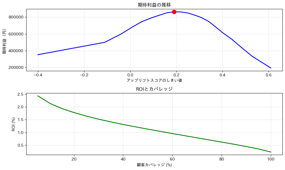
これらのグラフから、以下のような洞察が得られます。
- 上のグラフ(期待利益)は、しきい値が低すぎても高すぎても利益が下がることを示しています。最適な点(赤い点)でバランスが取れています。
- 下のグラフ(ROIとカバレッジ)は、少数の高スコア顧客に絞るほどROIは高くなりますが、機会損失も大きくなることを示しています。
実運用での実装パターン
分析結果を実際の施策に活用する方法は、大きく分けて2つのパターンがあります。
- バッチ型(定期的な処理)
- リアルタイム型(即時判定)
それぞれの特徴と実装方法を見ていきましょう。
バッチ型実装:定期的なリスト生成
多くの企業では、週次や月次でマーケティングキャンペーンを実施します。このような定期的な施策には、バッチ処理が適しています。
まず、バッチ処理の基本的な流れを理解しましょう。
- データ収集: 最新の顧客情報を収集
- スコア計算: アップリフトモデルでスコアを計算
- 対象選定: しきい値とビジネスルールに基づいて対象を選定
- リスト作成: 施策実施用のリストを生成
- 実行と記録: 施策を実行し、結果を記録
では、実際にシンプルなバッチ処理システムを実装してみましょう。
バッチ処理のための関数を定義します。本来はデータベースからデータを取得し実施しますが、ここでは簡易的に手元にあるデータで実施します。
以下、コードです。
import datetime
import os

# バッチ処理クラスの定義(簡易版)
class SimpleBatchUpliftScoring:

    def __init__(self, model=None, threshold=0.05):
        """
        初期化

        Parameters:
        -----------
        model : object
            学習済みアップリフトモデル
        threshold : float
            施策実施のしきい値
        """
        self.model = model
        self.threshold = threshold
        self.process_date = datetime.date.today()

    def extract_customer_data(self):
        """
        顧客データの抽出(実際はデータベースから取得)

        今回は既に読み込んだデータを使用します
        """
        print(f"[{datetime.datetime.now()}] データ抽出開始...")

        # 実際の実装では、ここでデータベースに接続して
        # 最新の顧客情報を取得します
        customer_data = data.copy()

        print(
            f"[{datetime.datetime.now()}] {len(customer_data)}件のデータを抽出しました"
        )
        return customer_data

    def score_customers(self, customer_data):
        """
        モデルを使用して顧客データにスコアを付与

        Parameters:
        -----------
        customer_data : DataFrame
            顧客データ

        Returns:
        --------
        scored_data : DataFrame
            スコアが付与された顧客データ
        """
        print(
            f"[{datetime.datetime.now()}] モデルを使用してスコアを計算中..."
        )

        # 特徴量を選択(モデルに必要なカラムのみ)
        features = customer_data[[
            'age',
            'purchase_history',
            'last_purchase_days',
            'email_open_rate'
        ]]

        # モデルでスコアを予測
        customer_data['uplift_score'] = self.model.predict_uplift(features)

        print(f"[{datetime.datetime.now()}] スコア計算完了")
        return customer_data

    def apply_business_rules(self, scored_data):
        """
        ビジネスルールの適用

        実際のビジネスでは、様々な制約条件があります。
        例えば:
        - 最近購入した顧客は除外
        - 高額顧客は別の施策対象とする
        - 予算の上限がある
        など
        """
        print(f"[{datetime.datetime.now()}] ビジネスルールを適用中...")

        # ルール1: アップリフトスコアがしきい値以上
        target_list = scored_data[scored_data['uplift_score'] >= self.threshold].copy()
        print(f"  - しきい値適用後: {len(target_list)}人")

        # ルール2: 最近購入した顧客は除外(7日以内)
        before_exclusion = len(target_list)
        target_list = target_list[target_list['last_purchase_days'] > 7]
        print(
            f"  - 最近購入者除外: {before_exclusion - len(target_list)}人を除外"
        )

        # ルール3: 予算制約(最大1000人)
        max_targets = 1000
        if len(target_list) > max_targets:
            # スコアの高い順に選択
            target_list = target_list.nlargest(max_targets, 'uplift_score')
            print(
                f"  - 予算制約により上位{max_targets}人に限定"
            )

        # キャンペーン情報を追加
        target_list['campaign_id'] = f"UPLIFT_{self.process_date}"
        target_list['process_date'] = self.process_date

        return target_list

    def save_results(self, target_list):
        """
        結果の保存

        CSVファイルとして保存します
        """
        # 保存用のディレクトリを作成
        os.makedirs('campaign_lists', exist_ok=True)

        # ファイル名に日付を含める
        filename = f"campaign_lists/targets_{self.process_date}.csv"

        # 必要な列のみを選択して保存
        save_columns = [
            'age',
            'purchase_history',
            'uplift_score',
            'campaign_id'
        ]
        target_list[save_columns].to_csv(filename, index=False)

        print(
            f"[{datetime.datetime.now()}] 結果を保存しました: {filename}"
        )
        return filename

    def generate_summary(self, target_list):
        """
        サマリーレポートの生成

        施策の概要を分かりやすくまとめます
        """
        summary = {
            '処理日': self.process_date,
            '対象人数': len(target_list),
            '平均アップリフトスコア': target_list['uplift_score'].mean(),
            '年齢層別人数': target_list.groupby(
                pd.cut(
                    target_list['age'],
                    bins=[0, 30, 40, 50, 100]
                )
            ).size().to_dict(),
        }

        return summary

    def run_batch(self):
        """
        バッチ処理の実行

        全体の処理フローを制御します
        """
        print(f"\n{'='*50}")
        print(f"バッチ処理開始: {self.process_date}")
        print(f"{'='*50}\n")

        try:
            # 1. データ抽出
            customer_data = self.extract_customer_data()

            # 2. モデルでスコアを計算
            scored_data = self.score_customers(customer_data)

            # 3. ビジネスルール適用
            target_list = self.apply_business_rules(scored_data)

            # 4. 結果保存
            saved_file = self.save_results(target_list)

            # 5. サマリー生成
            summary = self.generate_summary(target_list)

            print(f"\n[{datetime.datetime.now()}] バッチ処理完了!")
            print("\n=== 処理サマリー ===")
            for key, value in summary.items():
                print(f"{key}: {value}")

            return summary

        except Exception as e:
            print(f"エラーが発生しました: {str(e)}")
            raise
今回は、第1回の記事で作成したアップリフトモデルを読み込み利用します。
まずは、アップリフトモデルのクラスを定義します(第1回の記事のコード)。
以下、コードです。
from sklearn.ensemble import RandomForestClassifier

"""
Two-Model法によるアップリフト予測クラス
"""
class TwoModelUplift:

    def __init__(self, base_model=RandomForestClassifier):
        """
        初期化
        base_model: 使用する機械学習モデル(デフォルトはランダムフォレスト)
        """
        self.model_treatment = base_model(n_estimators=100, random_state=42)
        self.model_control = base_model(n_estimators=100, random_state=42)

    def fit(self, X, treatment, y):
        """
        モデルの学習
        X: 特徴量
        treatment: 施策実施フラグ(1=実施、0=非実施)
        y: 目的変数(購入フラグ)
        """
        # 処置群(クーポンあり)のデータ
        treatment_mask = treatment == 1
        X_treatment = X[treatment_mask]
        y_treatment = y[treatment_mask]

        # 対照群(クーポンなし)のデータ
        control_mask = treatment == 0
        X_control = X[control_mask]
        y_control = y[control_mask]

        # それぞれのモデルを学習
        self.model_treatment.fit(X_treatment, y_treatment)
        self.model_control.fit(X_control, y_control)

        print(f"処置群のサンプル数: {len(X_treatment)}")
        print(f"対照群のサンプル数: {len(X_control)}")

    def predict_uplift(self, X):
        """
        アップリフトスコアの予測
        X: 予測対象の特徴量
        """
        # 施策ありの場合の購入確率
        prob_treatment = self.model_treatment.predict_proba(X)[:, 1]

        # 施策なしの場合の購入確率
        prob_control = self.model_control.predict_proba(X)[:, 1]

        # アップリフトスコア = 施策ありの確率 - 施策なしの確率
        uplift_score = prob_treatment - prob_control

        return uplift_score
次に、第1回の記事で構築したアップリフトモデルを読み込みます。
以下、コードです。
import joblib

# モデルをロード
loaded_model = joblib.load('uplift_model.pkl')
このモデルを使い、バッチ処理を実施します。
以下、コードです。
# バッチ処理システムのインスタンスを作成
batch_processor = SimpleBatchUpliftScoring(
    model=loaded_model,
    threshold=optimal_threshold
)

# バッチ処理を実行
summary = batch_processor.run_batch()
以下、実行結果です。
==================================================
バッチ処理開始: 2025-08-23
==================================================

[2025-08-23 12:18:37.592152] データ抽出開始...
[2025-08-23 12:18:37.592340] 1500件のデータを抽出しました
[2025-08-23 12:18:37.592356] モデルを使用してスコアを計算中...
[2025-08-23 12:18:37.632113] スコア計算完了
[2025-08-23 12:18:37.632158] ビジネスルールを適用中...
  - しきい値適用後: 903人
  - 最近購入者除外: 206人を除外
[2025-08-23 12:18:37.975449] 結果を保存しました: campaign_lists/targets_2025-08-23.csv

[2025-08-23 12:18:37.982285] バッチ処理完了!

=== 処理サマリー ===
処理日: 2025-08-23
対象人数: 697
平均アップリフトスコア: 0.38276901004304165
年齢層別人数: {Interval(0, 30, closed='right'): 246, Interval(30, 40, closed='right'): 335, Interval(40, 50, closed='right'): 102, Interval(50, 100, closed='right'): 14}
リアルタイム型実装:即時判定システム
ECサイトやモバイルアプリでは、顧客がサイトを訪問した瞬間に「この顧客にクーポンを表示すべきか」を判断する必要があります。
このような場合は、リアルタイムAPIが適していますが、今回はJupyter Notebook上で動作する簡易的なリアルタイム判定システムを実装してみましょう。
そのための関数を定義します。
以下、コードです。
# リアルタイム判定システムの実装(簡易版)
class SimpleRealtimeUplift:

    def __init__(self, model, threshold=0.05):
        self.model = model  # 学習済みモデル
        self.threshold = threshold
        self.cache = {}  # 簡易的なキャッシュ
        self.prediction_log = []  # 予測ログ

    def extract_features(self, customer_info):
        """
        顧客情報から特徴量を抽出

        実際のシステムでは、データベースから追加情報を
        取得することもあります
        """
        # 必要な特徴量のデフォルト値
        default_values = {
            'age': 35,
            'purchase_history': 5,
            'last_purchase_days': 30,
            'email_open_rate': 0.2
        }

        # 顧客情報から特徴量を抽出(ない場合はデフォルト値を使用)
        features = {}
        for feature, default in default_values.items():
            features[feature] = customer_info.get(feature, default)

        return features

    def calculate_uplift_score(self, features):
        """
        アップリフトスコアの計算

        学習済みモデルを使用してスコアを計算
        """
        # 特徴量をデータフレーム形式に変換
        features_df = pd.DataFrame([features])

        # モデルでスコアを予測
        uplift_score = self.model.predict_uplift(features_df)[0]

        return uplift_score

    def should_show_campaign(self, customer_id, customer_info):
        """
        キャンペーンを表示すべきかを判定

        Parameters:
        -----------
        customer_id : str
            顧客ID
        customer_info : dict
            顧客情報

        Returns:
        --------
        result : dict
            判定結果
        """
        # キャッシュチェック(同じ顧客への重複計算を防ぐ)
        if customer_id in self.cache:
            return self.cache[customer_id]

        # 特徴量抽出
        features = self.extract_features(customer_info)

        # スコア計算
        uplift_score = self.calculate_uplift_score(features)

        # 判定
        should_target = uplift_score >= self.threshold

        # 結果を作成
        result = {
            'customer_id': customer_id,
            'uplift_score': uplift_score,
            'should_target': should_target,
            'threshold': self.threshold,
            'timestamp': datetime.datetime.now(),
            'features': features
        }

        # キャッシュに保存
        self.cache[customer_id] = result

        # ログに記録
        self.prediction_log.append(result)

        return result

    def get_statistics(self):
        """
        これまでの判定結果の統計を取得
        """
        if not self.prediction_log:
            return "まだ判定結果がありません"

        total_predictions = len(self.prediction_log)
        targeted = sum(1 for log in self.prediction_log if log['should_target'])

        stats = {
            '総判定数': total_predictions,
            'キャンペーン対象数': targeted,
            'キャンペーン対象率': targeted / total_predictions * 100,
            '平均アップリフトスコア': np.mean([log['uplift_score'] for log in self.prediction_log])
        }

        return stats
この関数を使い、リアルタイム判定をします。今回は、顧客データはテスト用に適当に設定したものを用いています。
今回は、第1回の記事で作成したアップリフトモデルを読み込み利用します。
以下、コードです。
# システムを初期化
realtime_system = SimpleRealtimeUplift(
    model=loaded_model,
    threshold=optimal_threshold
)

# テスト用の顧客データ
test_customers = [
    {
    	'customer_id': 'C001',
    	'age': 25,
    	'purchase_history': 2,
    	'last_purchase_days': 90
    },
    {
    	'customer_id': 'C002',
    	'age': 45,
    	'purchase_history': 10,
    	'last_purchase_days': 5
    },
    {
    	'customer_id': 'C003',
    	'age': 35,
    	'purchase_history': 5,
    	'last_purchase_days': 30
    },
    {
    	'customer_id': 'C004',
    	'age': 28,
    	'purchase_history': 1,
    	'last_purchase_days': 120
    },
    {
    	'customer_id': 'C005',
    	'age': 55,
    	'purchase_history': 15,
    	'last_purchase_days': 3
    }
]

print("=== リアルタイム判定のテスト ===\n")

# 各顧客に対して判定を実行
for customer in test_customers:
    result = realtime_system.should_show_campaign(
        customer['customer_id'],
        customer
    )

    print(f"顧客ID: {result['customer_id']}")
    print(f"  年齢: {result['features']['age']}歳")
    print(f"  購買履歴: {result['features']['purchase_history']}回")
    print(f"  アップリフトスコア: {result['uplift_score']:.3f}")
    print(f"  キャンペーン表示: {'はい' if result['should_target'] else 'いいえ'}")
    print()

# 統計情報を表示
print("\n=== 判定結果の統計 ===")
stats = realtime_system.get_statistics()
for key, value in stats.items():
    if isinstance(value, float):
        print(f"{key}: {value:.3f}")
    else:
        print(f"{key}: {value}")
以下、実行結果です。
=== リアルタイム判定のテスト ===

顧客ID: C001
  年齢: 25歳
  購買履歴: 2回
  アップリフトスコア: -0.060
  キャンペーン表示: いいえ

顧客ID: C002
  年齢: 45歳
  購買履歴: 10回
  アップリフトスコア: -0.030
  キャンペーン表示: いいえ

顧客ID: C003
  年齢: 35歳
  購買履歴: 5回
  アップリフトスコア: 0.260
  キャンペーン表示: はい

顧客ID: C004
  年齢: 28歳
  購買履歴: 1回
  アップリフトスコア: 0.080
  キャンペーン表示: いいえ

顧客ID: C005
  年齢: 55歳
  購買履歴: 15回
  アップリフトスコア: 0.270
  キャンペーン表示: はい


=== 判定結果の統計 ===
総判定数: 5
キャンペーン対象数: 2
キャンペーン対象率: 40.000
平均アップリフトスコア: 0.104
まとめ
今回は、アップリフト分析を実際のビジネスに導入するための方法について解説しました。
- しきい値の科学的な設定により、施策の費用対効果を最大化できることを学びました。数式に基づいた最適化により、勘や経験に頼らない意思決定が可能になります。
- バッチ処理とリアルタイム処理という2つの実装パターンを理解し、ビジネス要件に応じて使い分ける方法を習得しました。
アップリフト分析は、単なる分析手法ではなく、マーケティングの意思決定を根本的に変革する可能性を持っています。
データに基づいて「誰に」「何を」「いつ」提供すべきかを、データに基づいて判断することで、顧客満足度の向上とビジネス成果の最大化を同時に実現できます。
この3回のシリーズで学んだ知識を活かし、ぜひ実務での導入にチャレンジしてみてください。
最初は小さなパイロットプロジェクトから始めて、徐々に規模を拡大していくアプローチが成功への近道です。
データドリブンなマーケティングの新しい地平線を、一緒に切り開いていきましょう!