
TPOTは複数のパイプラインを構成し、評価します。
そのうち最も良いものを最適なパイプラインとして出力します。
人によっては、途中でどのようなパイプラインを構成し評価したのか、気になる方もいることでしょう。
実務的には、最終的に出力された最適なパイプラインではなく、2番目に良いパイプラインや3番目に良いパイプラインを使うこともあります。使い勝手や、解釈性、処理スピードなど色々な理由からです。
今回は、load_breast_cancer(乳がんの診断結果)の分類の例を使い、その生成されたパイプラインの評価結果を確認してみます。
Contents
取り急ぎ、TPOTでパイプライン生成
今回はソースコードの詳細な説明は省きます。
次のコードを実行し、TPOTのパイプラインを生成してください。
# ライブラリー読み込み
from tpot import TPOTClassifier
from sklearn.datasets import load_breast_cancer
from sklearn.model_selection import train_test_split
from sklearn.metrics import f1_score

# データセットを読み込み、Xに特徴量、yに目的変数を格納します
load_breast_cancer = load_breast_cancer()
X = load_breast_cancer.data
y = load_breast_cancer.target

# データセットを学習データ(X_train, y_train)とテストデータ(X_test, y_test)に分割します
X_train, X_test, y_train, y_test = train_test_split(
    X,
    y,
    train_size=0.75,
    test_size=0.25,
    random_state=42)

# TPOTの設定をします
tpot = TPOTClassifier(scoring='f1', # 評価に使うスコアを設定
                      generations=5,
                      population_size=50,
                      random_state=42,
                      verbosity=2, # 計算の経過を出力
                      periodic_checkpoint_folder='EvaluationResult' # パイプラインを評価指標とともに出力
                     )

# 学習します
tpot.fit(X_train, y_train)

# 最適化されたパイプラインを出力します
tpot.export('best_pipeline.py')

# テストデータで予測します
y_test_pred = tpot.predict(X_test)

# f1スコアを計算します
print('test f1 score=' + str(f1_score(y_true=y_test, y_pred=y_test_pred)))
以下、実行結果です。
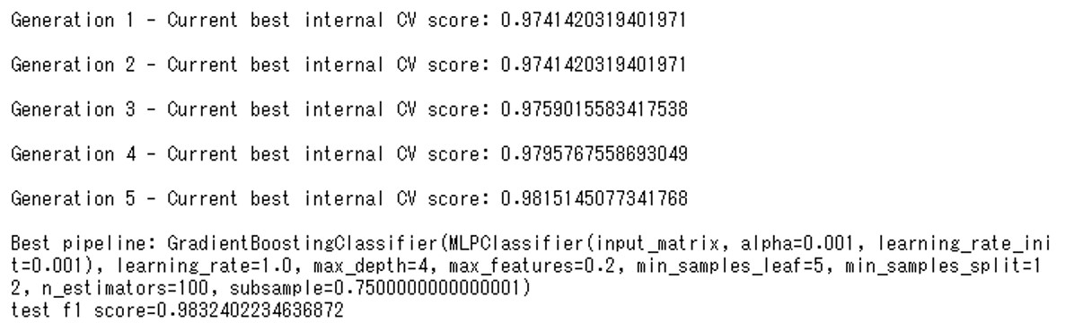
FスコアのCV score(クロスバリデーション・スコア)をみると、世代(Generation)を経るごとにスコアが良くなっていることがわかります。
- 第1世代のFスコアのCV Score:0.97414
- 第2世代のFスコアのCV Score:0.97414
- 第3世代のFスコアのCV Score:0.97590
- 第4世代のFスコアのCV Score:0.97957
- 第5世代のFスコアのCV Score:0.98151
それぞれの世代でどのようなパイプラインが構成されたか確認してみましょう。
ちなみに、CV scoreは交差検証を行ったときのスコアです。データセットをいくつかに分割し、一つをテストデータ、残りを学習データとして予測し、評価指標を算出します。予測及び評価を分割した回数分繰り返し、評価指標の平均をとったものがCV scoreで、このような検証方法を交差検証(Cross Varidation)と呼びます。過学習を防ぐためにこのような評価を行います。
パイプラインの途中経過の確認方法
TPOTClassifierのperiodic_checkpoint_folderパラメータにフォルダ名を指定することで途中の評価結果を出力できます。回帰問題に使うTPOTRegressorの場合も同様です。
ここではEvaluationResultフォルダに出力します。原則として1世代に1回、もしくは30秒に1回程度でパイプラインの評価結果が出力されます。世代間で変化がない場合には出力されない場合もあります。
先ほどのコードで実行すると、次のような4つのパイプラインが出力されると思います(人によっては5つ)。
- pipeline_gen_1_idx_0_2021.01.24_15-53-14.py … 第1世代の最適パイプライン
- pipeline_gen_3_idx_0_2021.01.24_15-55-03.py … 第3世代の最適パイプライン
- pipeline_gen_4_idx_0_2021.01.24_15-56-23.py … 第4世代の最適パイプライン
- pipeline_gen_5_idx_1_2021.01.24_15-57-46.py … 第5世代の最適パイプライン
実行したタイミングで出力されるファイルや結果は多少異なります。遺伝的アルゴリズムを使って最適なパイプラインを探索しているためです。
では、出力されたなかった第2世代を除いた、4つの世代(第1、第3、第4、第5)のそれぞれのファイルの中身を見てみましょう。
第1世代の最適パイプライン
第1世代のパイプラインは次のようになっていました。
import numpy as np
import pandas as pd
from sklearn.ensemble import GradientBoostingClassifier
from sklearn.model_selection import train_test_split

# NOTE: Make sure that the outcome column is labeled 'target' in the data file
tpot_data = pd.read_csv('PATH/TO/DATA/FILE', sep='COLUMN_SEPARATOR', dtype=np.float64)
features = tpot_data.drop('target', axis=1)
training_features, testing_features, training_target, testing_target = \
            train_test_split(features, tpot_data['target'], random_state=42)

# Average CV score on the training set was: 0.9741420319401971
exported_pipeline = GradientBoostingClassifier(learning_rate=1.0,
                                               max_depth=4,
                                               max_features=0.2,
                                               min_samples_leaf=5,
                                               min_samples_split=8,
                                               n_estimators=100,
                                               subsample=0.7500000000000001)
# Fix random state in exported estimator
if hasattr(exported_pipeline, 'random_state'):
    setattr(exported_pipeline, 'random_state', 42)

exported_pipeline.fit(training_features, training_target)
results = exported_pipeline.predict(testing_features)
12行目がこのパイプラインのCV scoreで、13行目から19行目が構成されたパイプラインです。
CV scoreは約0.974です。
パイプラインでは特徴量が元のデータそのまま、予測アルゴリズムとしてGradientBoostingClassifier(勾配ブースティング分類器)を使っています。
第3世代の最適パイプライン
第3世代のパイプラインは次のようになっていました。
import numpy as np
import pandas as pd
from sklearn.ensemble import GradientBoostingClassifier
from sklearn.model_selection import train_test_split
from sklearn.pipeline import make_pipeline, make_union
from tpot.builtins import StackingEstimator
from tpot.export_utils import set_param_recursive
from sklearn.preprocessing import FunctionTransformer
from copy import copy

# NOTE: Make sure that the outcome column is labeled 'target' in the data file
tpot_data = pd.read_csv('PATH/TO/DATA/FILE', sep='COLUMN_SEPARATOR', dtype=np.float64)
features = tpot_data.drop('target', axis=1)
training_features, testing_features, training_target, testing_target = \
            train_test_split(features, tpot_data['target'], random_state=42)

# Average CV score on the training set was: 0.9759015583417538
exported_pipeline = make_pipeline(
    make_union(
        FunctionTransformer(copy),
        FunctionTransformer(copy)
    ),
    GradientBoostingClassifier(learning_rate=0.1,
                               max_depth=9,
                               max_features=0.35000000000000003,
                               min_samples_leaf=20,
                               min_samples_split=17,
                               n_estimators=100,
                               subsample=0.5)
)
# Fix random state for all the steps in exported pipeline
set_param_recursive(exported_pipeline.steps, 'random_state', 42)

exported_pipeline.fit(training_features, training_target)
results = exported_pipeline.predict(testing_features)
17行目がCV score、18行~29行目がパイプラインです。
CV scoreは約0.976で、第1世代よりも良いスコアになっていることがわかります。
GradientBoostingClassifier(勾配ブースティング分類器)で学習および予測をします。
ただ、簡単なスタッキング処理をしています。スタッキングとは「複数の機械学習を積み重ねて精度を上げる手法」です。FunctionTransformer(copy)は,分類器の予測値とデータセットをマージし、そのマージして生成した特徴量(元のデータセット+分類器の予測値)でさらに学習します。要は、元のデータセットで学習し予測結果を出力し、その予測結果と元のデータセットを一緒にした新しいデータセットを作り、その新しいデータセットで学習し予測結果を出力し…… ということを繰り返します。
第4世代の最適パイプライン
第4世代のパイプラインは次のようになっていました。
import numpy as np
import pandas as pd
from sklearn.ensemble import GradientBoostingClassifier
from sklearn.model_selection import train_test_split

# NOTE: Make sure that the outcome column is labeled 'target' in the data file
tpot_data = pd.read_csv('PATH/TO/DATA/FILE', sep='COLUMN_SEPARATOR', dtype=np.float64)
features = tpot_data.drop('target', axis=1)
training_features, testing_features, training_target, testing_target = \
            train_test_split(features, tpot_data['target'], random_state=42)

# Average CV score on the training set was: 0.9795767558693049
exported_pipeline = GradientBoostingClassifier(learning_rate=0.5,
                                               max_depth=9,
                                               max_features=0.35000000000000003,
                                               min_samples_leaf=20,
                                               min_samples_split=17,
                                               n_estimators=100,
                                               subsample=0.5)
# Fix random state in exported estimator
if hasattr(exported_pipeline, 'random_state'):
    setattr(exported_pipeline, 'random_state', 42)

exported_pipeline.fit(training_features, training_target)
results = exported_pipeline.predict(testing_features)
12行目がCV score、13行~19行目がパイプラインです。
CV scoreは約0.980で第3世代よりも良くなっています。
パイプラインの構成ですが、特徴量は元のデータがそのまま使われており、予測アルゴリズムはGradientBoostingClassifier(勾配ブースティング分類器)が使われています。
第1世代と同じですが、パラメータの設定が異なっていることが分かります。
第5世代の最適パイプライン
第5世代のパイプラインは次のようになっていました。最後の世代です。
import numpy as np
import pandas as pd
from sklearn.ensemble import GradientBoostingClassifier
from sklearn.model_selection import train_test_split
from sklearn.neural_network import MLPClassifier
from sklearn.pipeline import make_pipeline, make_union
from tpot.builtins import StackingEstimator
from tpot.export_utils import set_param_recursive

# NOTE: Make sure that the outcome column is labeled 'target' in the data file
tpot_data = pd.read_csv('PATH/TO/DATA/FILE', sep='COLUMN_SEPARATOR', dtype=np.float64)
features = tpot_data.drop('target', axis=1)
training_features, testing_features, training_target, testing_target = \
            train_test_split(features, tpot_data['target'], random_state=42)

# Average CV score on the training set was: 0.9815145077341768
exported_pipeline = make_pipeline(
    StackingEstimator(estimator=MLPClassifier(alpha=0.001, learning_rate_init=0.001)),
    GradientBoostingClassifier(learning_rate=1.0,
                               max_depth=4,
                               max_features=0.2,
                               min_samples_leaf=5,
                               min_samples_split=12,
                               n_estimators=100,
                               subsample=0.7500000000000001)
)
# Fix random state for all the steps in exported pipeline
set_param_recursive(exported_pipeline.steps, 'random_state', 42)

exported_pipeline.fit(training_features, training_target)
results = exported_pipeline.predict(testing_features)
16行目がCV score、17行~26行目がパイプラインです。
CV scoreは約0.982で第4世代よりも良くなっています。
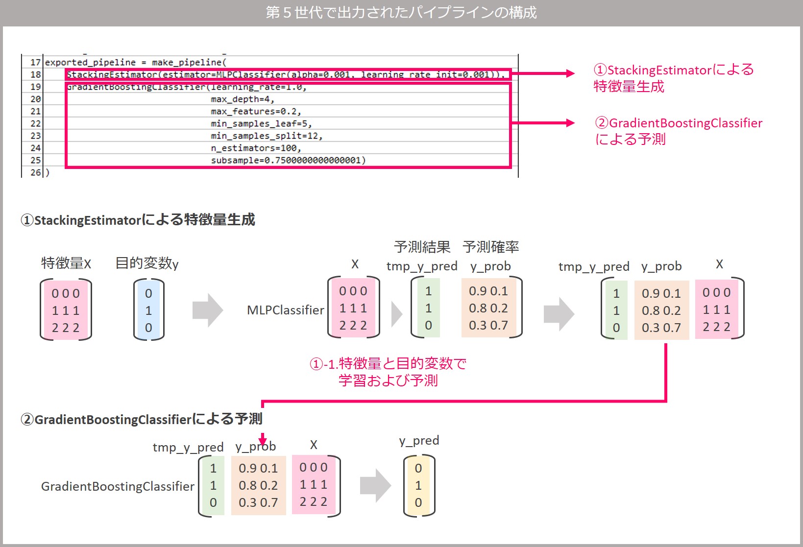
パイプラインはMLPClassifier(多層パーセプトロン分類器)とGradientBoostingClassifier(勾配ブースティング分類器)の2種類の分類器で構成され、StackingEstimatorを使ったスタッキング処理をしています。
StackingEstimatorはTPOT特有のEstimatorで、estimatorパラメータで指定した分類器であるMLPClassifier(多層パーセプトロン分類器)で予測した結果に、入力データを列方向に結合する関数です。その結合したデータを入力データとしてGradientBoostingClassifier(勾配ブースティング分類器)で学習および予測します。
分かりにくいと思いますので、以下に図解します。
最適パイプライン
以上が、各世代のパイプラインと評価結果でした。
最後に、全体を通して最適だと評価されたパイプラインを確認します。
ここではtpot.export()の引数に指定したbest_pipeline.pyファイルに最適パイプラインが出力されています。
では、最適なパイプライン(best_pipeline.py)を見てみます。
import numpy as np
import pandas as pd
from sklearn.ensemble import GradientBoostingClassifier
from sklearn.model_selection import train_test_split
from sklearn.neural_network import MLPClassifier
from sklearn.pipeline import make_pipeline, make_union
from tpot.builtins import StackingEstimator
from tpot.export_utils import set_param_recursive

# NOTE: Make sure that the outcome column is labeled 'target' in the data file
tpot_data = pd.read_csv('PATH/TO/DATA/FILE', sep='COLUMN_SEPARATOR', dtype=np.float64)
features = tpot_data.drop('target', axis=1)
training_features, testing_features, training_target, testing_target = \
            train_test_split(features, tpot_data['target'], random_state=42)

# Average CV score on the training set was: 0.9815145077341768
exported_pipeline = make_pipeline(
    StackingEstimator(estimator=MLPClassifier(alpha=0.001, learning_rate_init=0.001)),
    GradientBoostingClassifier(learning_rate=1.0,
                               max_depth=4,
                               max_features=0.2,
                               min_samples_leaf=5,
                               min_samples_split=12,
                               n_estimators=100,
                               subsample=0.7500000000000001)
)
# Fix random state for all the steps in exported pipeline
set_param_recursive(exported_pipeline.steps, 'random_state', 42)

exported_pipeline.fit(training_features, training_target)
results = exported_pipeline.predict(testing_features)
16行目がCV score、17行~26行目がパイプラインです。第5世代で出力されたパイプラインと一致することがわかります。
すべてのパイプラインを確認するには
今回は出力されたパイプラインだけを確認しました。
すべてのパイプラインを確認したい場合は、tpot.evaluated_individuals_を使うことで可能です。
例えば次のコードを使ってパイプラインや各CV scoreを出力することができます。
for k,v in tpot.evaluated_individuals_.items():
    print('------------------------------')
    print('generation=' + str(v['generation']))               # 世代数を表示
    print('internal_cv_score=' + str(v['internal_cv_score'])) # CVスコアを表示
    print(tpot.clean_pipeline_string(k))                      # パイプラインの文字列を成型
実行結果です。(結果が長いので途中で省略しています)
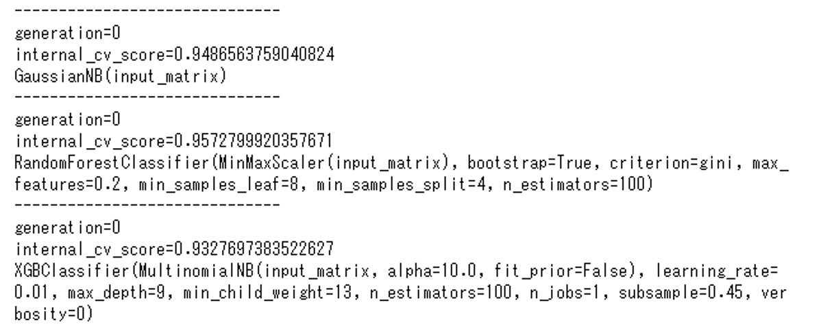
簡単にコードについて補足説明します。
TPOTが検討したパイプラインの情報はtpot.evaluated_individuals_に辞書形式で格納されています。辞書のキーがパイプラインを示す文字列になっており、値に入れ子で世代などの情報が入っています。
for文でキーと値を順に取り出して、print文で中身を表示しています。
tpot.evaluated_individuals_に格納されているキーの文字列のままではパイプラインを読み解きづらいので、tpot.clean_pipeline_string関数で読みやすい形式に変換しています。generasionに世代数、internal_cv_scoreにそのパイプラインのCV scoreが格納されています。
次回
次回は、パイプラインの評価に使える指標について説明します。